Hunting Performance in Python Code – Part 3. CPU Profiling (scripts)

In this post I will talk about some tools that can help us solve another painful problem in Python: profiling CPU usage.

CPU profiling means measuring the performance of our code by analyzing the way CPU executes the code. This translates to finding the hot spots in our code and see how we can deal with them.

We will see next how you can trace the CPU usage used by your Python scripts. We will focus on the following profilers (click them to go to the corresponding section in this blog):

• cProfile
• line_profiler
• pprofile
• vprof

Series index

The links below will go live once the posts are released:

1. Setup
2. Memory Profiling
3. CPU Profiling – Python Scripts
4. CPU Profiling – Python Interpreter

---

Measuring CPU Usage

For this post I will use mostly the same script as the one used in the memory analysis posts, and you can see it bellow or here.

	import time
	def primes(n):
	if n == 2:
	return [2]
	elif n < 2:
	return []
	s = []
	for i in range(3, n+1):
	if i % 2 != 0:
	s.append(i)
	mroot = n ** 0.5
	half = (n + 1) / 2 – 1
	i = 0
	m = 3
	while m <= mroot:
	if s[i]:
	j = (m * m – 3) / 2
	s[j] = 0
	while j < half:
	s[j] = 0
	j += m
	i = i + 1
	m = 2 * i + 3
	l = [2]
	for x in s:
	if x:
	l.append(x)
	return l
	def benchmark():
	start = time.time()
	for _ in xrange(40):
	count = len(primes(1000000))
	end = time.time()
	print "Benchmark duration: %r seconds" % (end-start)
	benchmark()

view raw

03.primes-v1.py

hosted with ❤ by GitHub

Also, remember that on PyPy2, you need to use a pip version that works with it:

pypy -m ensure pip

and anything else will be installed using:

pypy -m pip install

cProfile

One of the most used tools when talking about CPU profiling is cProfile, mainly because it comes builtin in CPython2 and PyPy2. It is a deterministic profiler, meaning that it will collect a set of statistic data when running our workload, such as execution count or execution time of various portions of our code. Furthermore, cProfile has a lower overhead on a system than other builtin profilers (profile or hotshot).

The usage is fairy simple when using CPython2:

python -m cProfile 03.primes-v1.py

If you are using PyPy2:

pypy -m cProfile 03.primes-v1.py

And the output of this is as follows:

	Benchmark duration: 30.11158514022827 seconds
	23139965 function calls in 30.112 seconds
	Ordered by: standard name
	ncalls tottime percall cumtime percall filename:lineno(function)
	1 0.000 0.000 30.112 30.112 03.primes.py:1(<module>)
	40 19.760 0.494 29.896 0.747 03.primes.py:3(primes)
	1 0.216 0.216 30.112 30.112 03.primes.py:31(benchmark)
	40 0.000 0.000 0.000 0.000 {len}
	23139840 6.683 0.000 6.683 0.000 {method 'append' of 'list' objects}
	1 0.000 0.000 0.000 0.000 {method 'disable' of '_lsprof.Profiler' objects}
	40 3.453 0.086 3.453 0.086 {range}
	2 0.000 0.000 0.000 0.000 {time.time}

view raw

03.cProfile.out

hosted with ❤ by GitHub

Even with this text output, it is straightforward to see that a lot of times our script calls the list.append method.

We can see the cProfile output in a graphical way if we use gprof2dot. To use it, we must first install graphviz as a requirement and after that the package itself. On Ubuntu give the commands:

apt-get install graphviz
pip install gprof2dot

We run our script again:

python -m cProfile -o output.pstats 03.primes-v1.py
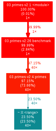
gprof2dot -f pstats output.pstats | dot -Tpng -o output.png

And we get the following output.png file:

More easier to see everything this way. Let’s take a closer look at what it outputs. You see a callgraph of functions from your script. In each square you see line by line:

• On the first line: the Python filename, the line number and the method name
• On the second line: the percentage of global time that this square uses
• On the third line: in brackets, the percentage of global time spent in the method itself
• On the fourth line: the number of calls made

For example, in the third red square from top, the method primes takes 98.28% of the time, with 65.44% doing something inside it, and it was called 40 times. The rest of the time is spent in the list.append(22.33%) and range(11.51%) methods from Python.

Being a simple script, we just have to re-write our script to not use so many appends, and it becomes like this:

	import time
	def primes(n):
	if n==2:
	return [2]
	elif n<2:
	return []
	s=range(3,n+1,2)
	mroot = n ** 0.5
	half=(n+1)/2-1
	i=0
	m=3
	while m <= mroot:
	if s[i]:
	j=(m*m-3)/2
	s[j]=0
	while j<half:
	s[j]=0
	j+=m
	i=i+1
	m=2*i+3
	return [2]+[x for x in s if x]
	def benchmark():
	start = time.time()
	for _ in xrange(40):
	count = len(primes(1000000))
	end = time.time()
	print "Benchmark duration: %r seconds" % (end-start)
	benchmark()

view raw

03.primes-v2.py

hosted with ❤ by GitHub

If we measure the time of our script before and now with CPython2:

python 03.primes-v1.py
Benchmark duration: 15.768115043640137 seconds

python 03.primes-v2.py
Benchmark duration: 6.56312108039856 seconds

Also with PyPy2:

pypy 03.primes-v1.py
Benchmark duration: 1.4009230136871338 seconds

pypy 03.primes-v2.py
Benchmark duration: 0.4542720317840576 seconds

We get a good 2.4X improvement with CPython2 and 3.1X with PyPy2. Not bad. And the cProfile callgraph:

You can also use cProfile in a programatic way, such as:

import cProfile
 
pr = cProfile.Profile()
pr.enable()
 
function_to_measure()

pr.disable()
pr.print_stats(sort='time')

This is useful in some scenarios, such as multiprocess performance measurents. More can be seen here.

line_profiler

This profiler provides information at line level on a workload. It is implemented in C using Cython and has a small overhead when comparing it to cProfile.

The source code repo can be found here and the PyPI page here. It has quite an overhead, compared to cProfile, taking 12X more time to get a profile.

To use it, you need first to add it via pip: pip install pip install Cython ipython==5.4.1 line_profiler (CPython2). One major downside of this profiler, is that it does not have support for PyPy.

Just like when using memory_profiler, you need to add a decorator to the function you want to be profiled. In our case, you need to add @profile before the definition of our primes function in 03.primes-v1.py. Then call it like this:

kernprof -l 03.primes-v1.py
python -m line_profiler 03.primes-v1.py.lprof

You will get an output like this:

	Timer unit: 1e-06 s
	Total time: 181.595 s
	File: 03.primes-v1.py
	Function: primes at line 3
	Line # Hits Time Per Hit % Time Line Contents
	==============================================================
	3 @profile
	4 def primes(n):
	5 40 107 2.7 0.0 if n == 2:
	6 return [2]
	7 40 49 1.2 0.0 elif n < 2:
	8 return []
	9 40 44 1.1 0.0 s = []
	10 39999960 34410114 0.9 18.9 for i in range(3, n+1):
	11 39999920 29570173 0.7 16.3 if i % 2 != 0:
	12 19999960 14976433 0.7 8.2 s.append(i)
	13 40 329 8.2 0.0 mroot = n ** 0.5
	14 40 82 2.0 0.0 half = (n + 1) / 2 – 1
	15 40 46 1.1 0.0 i = 0
	16 40 30 0.8 0.0 m = 3
	17 20000 17305 0.9 0.0 while m <= mroot:
	18 19960 16418 0.8 0.0 if s[i]:
	19 6680 6798 1.0 0.0 j = (m * m – 3) / 2
	20 6680 6646 1.0 0.0 s[j] = 0
	21 32449400 22509523 0.7 12.4 while j < half:
	22 32442720 26671867 0.8 14.7 s[j] = 0
	23 32442720 22913591 0.7 12.6 j += m
	24 19960 15078 0.8 0.0 i = i + 1
	25 19960 16170 0.8 0.0 m = 2 * i + 3
	26 40 87 2.2 0.0 l = [2]
	27 20000000 14292643 0.7 7.9 for x in s:
	28 19999960 13753547 0.7 7.6 if x:
	29 3139880 2417421 0.8 1.3 l.append(x)
	30 40 33 0.8 0.0 return l

view raw

03.line_profiler.out

hosted with ❤ by GitHub

We see that the two loops that call repeatedly list.append take the most time from our script.

pprofile

According to the author, pprofile is a “line-granularity, thread-aware deterministic and statistic pure-python profiler”. 

It is inspired from line_profiler, fixes a lot of disadvantage, but because it is written entirely in Python, it can be used successfully with PyPy also. Compared to cProfile, an analysis takes 28X more time when using CPython, and 10X more time when using PyPy but also the level of detail is much more granular.

And we have support for PyPy! An addition to it, it’s that it has support for profiling threads, which may come handy in various situations.

To use it, you need first to add it via pip: pip install pprofile (CPython2) / pypy -m pip install pprofile (PyPy) and then call it like this:

pprofile 03.primes-v1.py

The output is different than what we seen before and we get something like this:

	Benchmark duration: 886.8774709701538 seconds
	Command line: ['03.primes-v1.py']
	Total duration: 886.878s
	File: 03.primes-v1.py
	File duration: 886.878s (100.00%)
	Line #| Hits| Time| Time per hit| %|Source code
	——+———-+————-+————-+——-+———–
	1| 2| 7.10487e-05| 3.55244e-05| 0.00%|import time
	2| 0| 0| 0| 0.00%|
	3| 0| 0| 0| 0.00%|
	4| 41| 0.00029397| 7.17e-06| 0.00%|def primes(n):
	5| 40| 0.000231266| 5.78165e-06| 0.00%| if n == 2:
	6| 0| 0| 0| 0.00%| return [2]
	7| 40| 0.000178337| 4.45843e-06| 0.00%| elif n < 2:
	8| 0| 0| 0| 0.00%| return []
	9| 40| 0.000188112| 4.70281e-06| 0.00%| s = []
	10| 39999960| 159.268| 3.98171e-06| 17.96%| for i in range(3, n+1):
	11| 39999920| 152.924| 3.82312e-06| 17.24%| if i % 2 != 0:
	12| 19999960| 76.2135| 3.81068e-06| 8.59%| s.append(i)
	13| 40| 0.00147367| 3.68416e-05| 0.00%| mroot = n ** 0.5
	14| 40| 0.000319004| 7.9751e-06| 0.00%| half = (n + 1) / 2 – 1
	15| 40| 0.000220776| 5.51939e-06| 0.00%| i = 0
	16| 40| 0.000243902| 6.09756e-06| 0.00%| m = 3
	17| 20000| 0.0777466| 3.88733e-06| 0.01%| while m <= mroot:
	18| 19960| 0.0774016| 3.87784e-06| 0.01%| if s[i]:
	19| 6680| 0.0278566| 4.17015e-06| 0.00%| j = (m * m – 3) / 2
	20| 6680| 0.0275929| 4.13067e-06| 0.00%| s[j] = 0
	21| 32449400| 114.858| 3.5396e-06| 12.95%| while j < half:
	22| 32442720| 120.841| 3.72475e-06| 13.63%| s[j] = 0
	23| 32442720| 114.432| 3.5272e-06| 12.90%| j += m
	24| 19960| 0.0749919| 3.75711e-06| 0.01%| i = i + 1
	25| 19960| 0.0765574| 3.83554e-06| 0.01%| m = 2 * i + 3
	26| 40| 0.000222206| 5.55515e-06| 0.00%| l = [2]
	27| 20000000| 68.8031| 3.44016e-06| 7.76%| for x in s:
	28| 19999960| 67.9391| 3.39696e-06| 7.66%| if x:
	29| 3139880| 10.9989| 3.50295e-06| 1.24%| l.append(x)
	30| 40| 0.000155687| 3.89218e-06| 0.00%| return l
	31| 0| 0| 0| 0.00%|
	32| 0| 0| 0| 0.00%|
	33| 2| 8.10623e-06| 4.05312e-06| 0.00%|def benchmark():
	34| 1| 5.00679e-06| 5.00679e-06| 0.00%| start = time.time()
	35| 41| 0.00101089| 2.4656e-05| 0.00%| for _ in xrange(40):
	36| 40| 0.232263| 0.00580657| 0.03%| count = len(primes(1000000))
	(call)| 40| 886.644| 22.1661| 99.97%|# 03.primes-v1.py:4 primes
	37| 1| 5.96046e-06| 5.96046e-06| 0.00%| end = time.time()
	38| 1| 0.000678062| 0.000678062| 0.00%| print "Benchmark duration: %r seconds" % (end-start)
	39| 0| 0| 0| 0.00%|
	40| 0| 0| 0| 0.00%|
	41| 1| 5.79357e-05| 5.79357e-05| 0.00%|benchmark()
	(call)| 1| 886.878| 886.878|100.00%|# 03.primes-v1.py:33 benchmark

view raw

03.pprofile.out

hosted with ❤ by GitHub

We now can see everything in more detail. Let’s go a bit through the output. You get the entire output of the script, and in front of each line you see the number of calls made to it, how much time was spent running it (in seconds), the time per each call and the percentage of the global time spent running it. Also, pprofile adds extra lines to our output (like line 44 and 50, which start with (call)), with the cumulated metrics.

Again, we see that the two loops that call repeatedly list.append take the most time from our script.

vprof

vprof is a Python profiler providing rich and interactive visualizations for various Python program characteristics such as running time and memory usage. It is a graphical one, based on Node.JS to display the results in a webpage.

With it, you can see one or all of the following, related to Python scripts:

• CPU flame graph
• code profiling
• memory graph
• code heatmap

To use it, you need first to add it via pip: pip install vprof (CPython2) / pypy -m pip install vprof (PyPy) and then call it like this:

On CPython2, to display the code heatmap (first call below) and the code profiling (second call below):

vprof -c h 03.primes-v1.py
vprof -c p 03.primes-v1.py

On PyPy, to display the code heatmap (first call below) and the code profiling (second call below):

pypy -m vprof -c h 03.primes-v1.py
pypy -m vprof -c p 03.primes-v1.py

On each case, you will see the following for the code heatmap

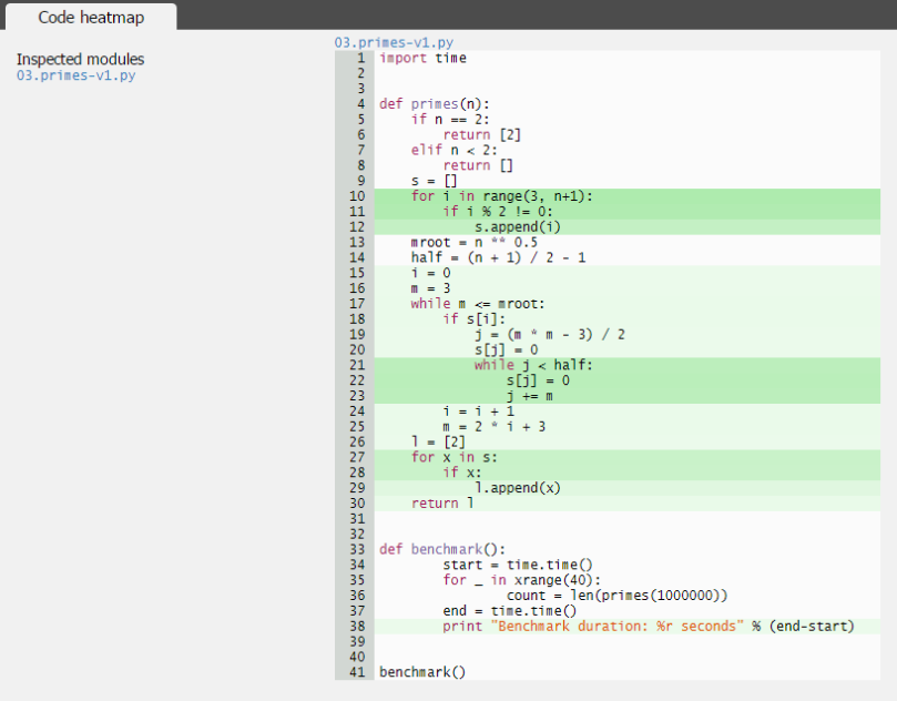
and the following for the code profiling.

The results are seen in a graphical way, and we can hover the mouse or click each line for more info.

Again, we see that the two loops that call repeatedly list.append take the most time from our script.

---

By Alecsandru Patrascu, alecsandru.patrascu [at] rinftech [dot] com